import pandas as pd
# to display all columns
pd.set_option('display.max.columns', None)
# to display the entire contents of a cell
pd.set_option('display.max_colwidth', None)
import numpy as np

import matplotlib.pyplot as plt
import seaborn as sns
%matplotlib inline
plt.style.use("ggplot")Libraries
mvc = pd.read_csv("../datasets/nypd_mvc_2018.csv")
mvc.head()| unique_key | date | time | borough | location | on_street | cross_street | off_street | pedestrians_injured | cyclist_injured | motorist_injured | total_injured | pedestrians_killed | cyclist_killed | motorist_killed | total_killed | vehicle_1 | vehicle_2 | vehicle_3 | vehicle_4 | vehicle_5 | cause_vehicle_1 | cause_vehicle_2 | cause_vehicle_3 | cause_vehicle_4 | cause_vehicle_5 | |
|---|---|---|---|---|---|---|---|---|---|---|---|---|---|---|---|---|---|---|---|---|---|---|---|---|---|---|
| 0 | 3869058 | 2018-03-23 | 21:40 | MANHATTAN | (40.742832, -74.00771) | WEST 15 STREET | 10 AVENUE | NaN | 0 | 0 | 0 | 0.0 | 0 | 0 | 0 | 0.0 | PASSENGER VEHICLE | NaN | NaN | NaN | NaN | Following Too Closely | Unspecified | NaN | NaN | NaN |
| 1 | 3847947 | 2018-02-13 | 14:45 | BROOKLYN | (40.623714, -73.99314) | 16 AVENUE | 62 STREET | NaN | 0 | 0 | 0 | 0.0 | 0 | 0 | 0 | 0.0 | SPORT UTILITY / STATION WAGON | DS | NaN | NaN | NaN | Backing Unsafely | Unspecified | NaN | NaN | NaN |
| 2 | 3914294 | 2018-06-04 | 0:00 | NaN | (40.591755, -73.9083) | BELT PARKWAY | NaN | NaN | 0 | 0 | 1 | 1.0 | 0 | 0 | 0 | 0.0 | Station Wagon/Sport Utility Vehicle | Sedan | NaN | NaN | NaN | Following Too Closely | Unspecified | NaN | NaN | NaN |
| 3 | 3915069 | 2018-06-05 | 6:36 | QUEENS | (40.73602, -73.87954) | GRAND AVENUE | VANLOON STREET | NaN | 0 | 0 | 0 | 0.0 | 0 | 0 | 0 | 0.0 | Sedan | Sedan | NaN | NaN | NaN | Glare | Passing Too Closely | NaN | NaN | NaN |
| 4 | 3923123 | 2018-06-16 | 15:45 | BRONX | (40.884727, -73.89945) | NaN | NaN | 208 WEST 238 STREET | 0 | 0 | 0 | 0.0 | 0 | 0 | 0 | 0.0 | Station Wagon/Sport Utility Vehicle | Sedan | NaN | NaN | NaN | Turning Improperly | Unspecified | NaN | NaN | NaN |
A summary of the columns and their data is below:
unique_key: A unique identifier for each collision.date, time: Date and time of the collision.borough: The borough, or area of New York City, where the collision occurred.location: Latitude and longitude coordinates for the collision.on_street, cross_street, off_street: Details of the street or intersection where the collision occurred.pedestrians_injured: Number of pedestrians who were injured.cyclist_injured: Number of people traveling on a bicycle who were injured.motorist_injured: Number of people traveling in a vehicle who were injured.total_injured: Total number of people injured.pedestrians_killed: Number of pedestrians who were killed.cyclist_killed: Number of people traveling on a bicycle who were killed.motorist_killed: Number of people traveling in a vehicle who were killed.total_killed: Total number of people killed.vehicle_1 through vehicle_5: Type of each vehicle involved in the accident.cause_vehicle_1 through cause_vehicle_5: Contributing factor for each vehicle in the accident.
Missing Values
mvc.isna().sum()unique_key 0
date 0
time 0
borough 20646
location 3885
on_street 13961
cross_street 29249
off_street 44093
pedestrians_injured 0
cyclist_injured 0
motorist_injured 0
total_injured 1
pedestrians_killed 0
cyclist_killed 0
motorist_killed 0
total_killed 5
vehicle_1 355
vehicle_2 12262
vehicle_3 54352
vehicle_4 57158
vehicle_5 57681
cause_vehicle_1 175
cause_vehicle_2 8692
cause_vehicle_3 54134
cause_vehicle_4 57111
cause_vehicle_5 57671
dtype: int64To give us a better picture of the null values in the data, let’s calculate the percentage of null values in each column.
null_df = pd.DataFrame({'null_counts':mvc.isna().sum(), 'null_pct':mvc.isna().sum()/mvc.shape[0] * 100}).T.astype(int).T
null_df| null_counts | null_pct | |
|---|---|---|
| unique_key | 0 | 0 |
| date | 0 | 0 |
| time | 0 | 0 |
| borough | 20646 | 35 |
| location | 3885 | 6 |
| on_street | 13961 | 24 |
| cross_street | 29249 | 50 |
| off_street | 44093 | 76 |
| pedestrians_injured | 0 | 0 |
| cyclist_injured | 0 | 0 |
| motorist_injured | 0 | 0 |
| total_injured | 1 | 0 |
| pedestrians_killed | 0 | 0 |
| cyclist_killed | 0 | 0 |
| motorist_killed | 0 | 0 |
| total_killed | 5 | 0 |
| vehicle_1 | 355 | 0 |
| vehicle_2 | 12262 | 21 |
| vehicle_3 | 54352 | 93 |
| vehicle_4 | 57158 | 98 |
| vehicle_5 | 57681 | 99 |
| cause_vehicle_1 | 175 | 0 |
| cause_vehicle_2 | 8692 | 15 |
| cause_vehicle_3 | 54134 | 93 |
| cause_vehicle_4 | 57111 | 98 |
| cause_vehicle_5 | 57671 | 99 |
About a third of the columns have no null values, with the rest ranging from less than 1% to 99%! To make things easier, let’s start by looking at the group of columns that relate to people killed in collisions.
null_df.loc[[column for column in mvc.columns if "killed" in column]]| null_counts | null_pct | |
|---|---|---|
| pedestrians_killed | 0 | 0 |
| cyclist_killed | 0 | 0 |
| motorist_killed | 0 | 0 |
| total_killed | 5 | 0 |
We can see that each of the individual categories have no missing values, but the total_killed column has five missing values.
If you think about it, the total number of people killed should be the sum of each of the individual categories. We might be able to “fill in” the missing values with the sums of the individual columns for that row.
Important
The technical name for filling in a missing value with a replacement value is called imputation.
Verifying the total columns
killed = mvc[[col for col in mvc.columns if 'killed' in col]].copy()
killed_manual_sum = killed.iloc[:, :3].sum(axis="columns")
killed_mask = killed_manual_sum != killed.total_killed
killed_non_eq = killed[killed_mask]
killed_non_eq| pedestrians_killed | cyclist_killed | motorist_killed | total_killed | |
|---|---|---|---|---|
| 3508 | 0 | 0 | 0 | NaN |
| 20163 | 0 | 0 | 0 | NaN |
| 22046 | 0 | 0 | 1 | 0.0 |
| 48719 | 0 | 0 | 0 | NaN |
| 55148 | 0 | 0 | 0 | NaN |
| 55699 | 0 | 0 | 0 | NaN |
Filling and Verifying the killed and the injured data
The killed_non_eq dataframe has six rows. We can categorize these into two categories:
- Five rows where the
total_killedis not equal to the sum of the other columns because the total value is missing. - One row where the
total_killedis less than the sum of the other columns.
From this, we can conclude that filling null values with the sum of the columns is a fairly good choice for our imputation, given that only six rows out of around 58,000 don’t match this pattern.
We’ve also identified a row that has suspicious data - one that doesn’t sum correctly. Once we have imputed values for all rows with missing values for total_killed, we’ll mark this suspect row by setting its value to NaN.
# fix the killed values
killed['total_killed'] = killed['total_killed'].mask(killed['total_killed'].isnull(), killed_manual_sum)
killed['total_killed'] = killed['total_killed'].mask(killed['total_killed'] != killed_manual_sum, np.nan)

# Create an injured dataframe and manually sum values
injured = mvc[[col for col in mvc.columns if 'injured' in col]].copy()
injured_manual_sum = injured.iloc[:,:3].sum(axis=1)

injured['total_injured'] = injured.total_injured.mask(injured.total_injured.isnull(), injured_manual_sum)

injured['total_injured'] = injured.total_injured.mask(injured.total_injured != injured_manual_sum, np.nan)
Let’s summarize the count of null values before and after our changes:
summary = {
    'injured': [
        mvc['total_injured'].isnull().sum(),
        injured['total_injured'].isnull().sum()
    ],
    'killed': [
        mvc['total_killed'].isnull().sum(),
        killed['total_killed'].isnull().sum()
    ]
}
pd.DataFrame(summary, index=['before','after'])| injured | killed | |
|---|---|---|
| before | 1 | 5 |
| after | 21 | 1 |
For the total_killed column, the number of values has gone down from 5 to 1. For the total_injured column, the number of values has actually gone up — from 1 to 21. This might sound like we’ve done the opposite of what we set out to do, but what we’ve actually done is fill all the null values and identify values that have suspect data. This will make any analysis we do on this data more accurate in the long run.
Let’s assign the values from the killed and injured dataframe back to the main mvc dataframe:
mvc['total_injured']=injured.total_injured
mvc['total_killed']=killed.total_killed
Visualizing the missing data with plots
Earlier, we used a table of numbers to understand the number of missing values in our dataframe. A different approach we can take is to use a plot to visualize the missing values. The function below uses seaborn.heatmap() to represent null values as dark squares and non-null values as light squares:
def plot_null_matrix(df, figsize=(20,15)):
    """Plot null values as light squares and non-null values as dark squares"""
    plt.figure(figsize=figsize)
    df_null = df.isnull()
    sns.heatmap(~df_null, cbar=False, yticklabels=False)
    plt.xticks(rotation=90, size="x-large")
    plt.show()
Let’s look at how the function works by using it to plot just the first row of our mvc dataframe. We’ll display the first row as a table immediately below so it’s easy to compare:
plot_null_matrix(mvc.head(1), figsize=(20,2))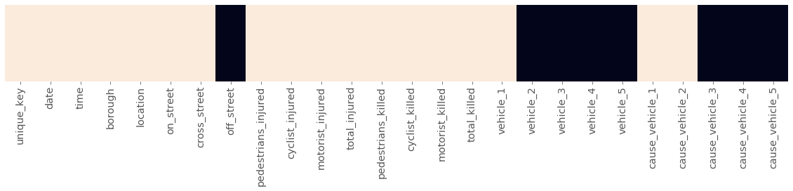
mvc.head(1)| unique_key | date | time | borough | location | on_street | cross_street | off_street | pedestrians_injured | cyclist_injured | motorist_injured | total_injured | pedestrians_killed | cyclist_killed | motorist_killed | total_killed | vehicle_1 | vehicle_2 | vehicle_3 | vehicle_4 | vehicle_5 | cause_vehicle_1 | cause_vehicle_2 | cause_vehicle_3 | cause_vehicle_4 | cause_vehicle_5 | |
|---|---|---|---|---|---|---|---|---|---|---|---|---|---|---|---|---|---|---|---|---|---|---|---|---|---|---|
| 0 | 3869058 | 2018-03-23 | 21:40 | MANHATTAN | (40.742832, -74.00771) | WEST 15 STREET | 10 AVENUE | NaN | 0 | 0 | 0 | 0.0 | 0 | 0 | 0 | 0.0 | PASSENGER VEHICLE | NaN | NaN | NaN | NaN | Following Too Closely | Unspecified | NaN | NaN | NaN |
Each value is represented by a light square, and each missing value is represented by a dark square.
Let’s look at what a plot matrix looks like for the whole dataframe:
plot_null_matrix(mvc)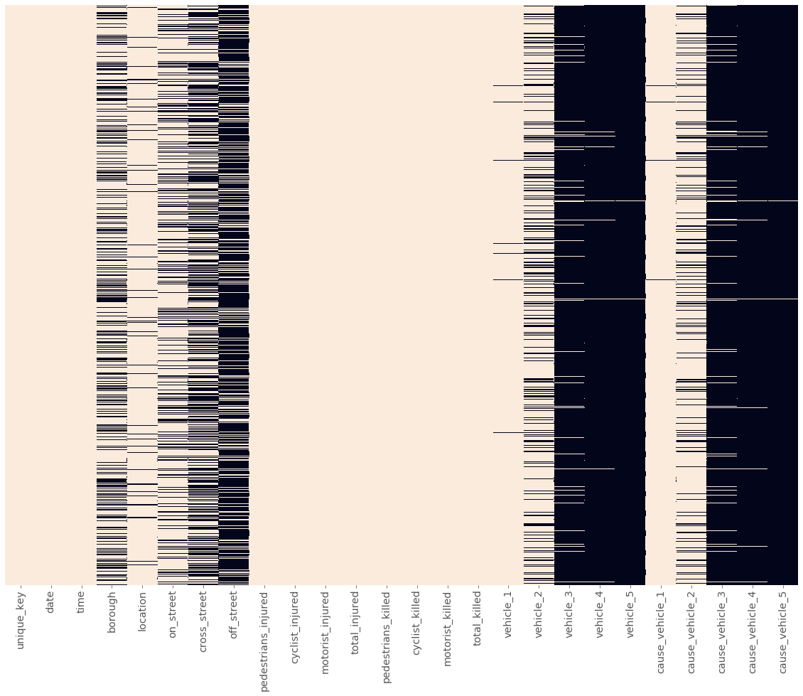
We can make some immediate interpretations about our dataframe:
- The first three columns have few to no missing values.
- The next five columns have missing values scattered throughout, with each column seeming to have its own density of missing values.
- The next eight columns are the
injuryandkilledcolumns we just cleaned, and only have a few missing values. - The last 10 columns seem to break into two groups of five, with each group of five having similar patterns of null/non-null values.
Let’s examine the pattern in the last 10 columns a little more closely. We can calculate the relationship between two sets of columns, known as correlation.
cols_with_missing_vals = mvc.columns[mvc.isnull().sum()>0]
missing_corr = mvc[cols_with_missing_vals].isnull().corr()
missing_corr| borough | location | on_street | cross_street | off_street | total_injured | total_killed | vehicle_1 | vehicle_2 | vehicle_3 | vehicle_4 | vehicle_5 | cause_vehicle_1 | cause_vehicle_2 | cause_vehicle_3 | cause_vehicle_4 | cause_vehicle_5 | |
|---|---|---|---|---|---|---|---|---|---|---|---|---|---|---|---|---|---|
| borough | 1.000000 | 0.190105 | -0.350190 | 0.409107 | 0.362189 | -0.002827 | 0.005582 | -0.018325 | -0.077516 | -0.061932 | -0.020406 | -0.010733 | -0.012115 | -0.058596 | -0.060542 | -0.020158 | -0.011348 |
| location | 0.190105 | 1.000000 | -0.073975 | -0.069719 | 0.084579 | -0.001486 | 0.015496 | -0.010466 | -0.033842 | -0.000927 | 0.004655 | -0.005797 | -0.003458 | -0.021373 | 0.000684 | 0.004604 | -0.004841 |
| on_street | -0.350190 | -0.073975 | 1.000000 | 0.557767 | -0.991030 | 0.006220 | -0.002344 | -0.001889 | 0.119647 | 0.020867 | 0.004172 | -0.002768 | 0.001307 | 0.087374 | 0.017426 | 0.002737 | -0.003107 |
| cross_street | 0.409107 | -0.069719 | 0.557767 | 1.000000 | -0.552763 | 0.002513 | 0.004112 | -0.017018 | 0.043799 | -0.049910 | -0.021137 | -0.012003 | -0.009102 | 0.031189 | -0.052159 | -0.022074 | -0.013455 |
| off_street | 0.362189 | 0.084579 | -0.991030 | -0.552763 | 1.000000 | -0.004266 | 0.002323 | 0.001812 | -0.121129 | -0.022404 | -0.004074 | 0.002492 | -0.001738 | -0.088187 | -0.019120 | -0.002580 | 0.002863 |
| total_injured | -0.002827 | -0.001486 | 0.006220 | 0.002513 | -0.004266 | 1.000000 | -0.000079 | 0.079840 | 0.025644 | -0.002757 | 0.002118 | 0.001073 | 0.131140 | 0.030082 | -0.002388 | 0.002188 | 0.001102 |
| total_killed | 0.005582 | 0.015496 | -0.002344 | 0.004112 | 0.002323 | -0.000079 | 1.000000 | -0.000327 | 0.008017 | 0.001057 | 0.000462 | 0.000234 | -0.000229 | 0.009888 | 0.001091 | 0.000477 | 0.000240 |
| vehicle_1 | -0.018325 | -0.010466 | -0.001889 | -0.017018 | 0.001812 | 0.079840 | -0.000327 | 1.000000 | 0.151516 | 0.019972 | 0.008732 | 0.004425 | 0.604281 | 0.180678 | 0.020624 | 0.009022 | 0.004545 |
| vehicle_2 | -0.077516 | -0.033842 | 0.119647 | 0.043799 | -0.121129 | 0.025644 | 0.008017 | 0.151516 | 1.000000 | 0.131813 | 0.057631 | 0.029208 | 0.106214 | 0.784402 | 0.132499 | 0.058050 | 0.029264 |
| vehicle_3 | -0.061932 | -0.000927 | 0.020867 | -0.049910 | -0.022404 | -0.002757 | 0.001057 | 0.019972 | 0.131813 | 1.000000 | 0.437214 | 0.221585 | 0.014000 | 0.106874 | 0.961316 | 0.448525 | 0.225067 |
| vehicle_4 | -0.020406 | 0.004655 | 0.004172 | -0.021137 | -0.004074 | 0.002118 | 0.000462 | 0.008732 | 0.057631 | 0.437214 | 1.000000 | 0.506810 | 0.006121 | 0.046727 | 0.423394 | 0.963723 | 0.515058 |
| vehicle_5 | -0.010733 | -0.005797 | -0.002768 | -0.012003 | 0.002492 | 0.001073 | 0.000234 | 0.004425 | 0.029208 | 0.221585 | 0.506810 | 1.000000 | 0.003102 | 0.023682 | 0.214580 | 0.490537 | 0.973664 |
| cause_vehicle_1 | -0.012115 | -0.003458 | 0.001307 | -0.009102 | -0.001738 | 0.131140 | -0.000229 | 0.604281 | 0.106214 | 0.014000 | 0.006121 | 0.003102 | 1.000000 | 0.131000 | 0.014457 | 0.006324 | 0.003186 |
| cause_vehicle_2 | -0.058596 | -0.021373 | 0.087374 | 0.031189 | -0.088187 | 0.030082 | 0.009888 | 0.180678 | 0.784402 | 0.106874 | 0.046727 | 0.023682 | 0.131000 | 1.000000 | 0.110362 | 0.048277 | 0.024322 |
| cause_vehicle_3 | -0.060542 | 0.000684 | 0.017426 | -0.052159 | -0.019120 | -0.002388 | 0.001091 | 0.020624 | 0.132499 | 0.961316 | 0.423394 | 0.214580 | 0.014457 | 0.110362 | 1.000000 | 0.437440 | 0.220384 |
| cause_vehicle_4 | -0.020158 | 0.004604 | 0.002737 | -0.022074 | -0.002580 | 0.002188 | 0.000477 | 0.009022 | 0.058050 | 0.448525 | 0.963723 | 0.490537 | 0.006324 | 0.048277 | 0.437440 | 1.000000 | 0.503805 |
| cause_vehicle_5 | -0.011348 | -0.004841 | -0.003107 | -0.013455 | 0.002863 | 0.001102 | 0.000240 | 0.004545 | 0.029264 | 0.225067 | 0.515058 | 0.973664 | 0.003186 | 0.024322 | 0.220384 | 0.503805 | 1.000000 |
Each value is between -1 and 1, and represents the relationship between two columns. A number close to 1 or -1 represents a strong relationship, where a number in the middle (close to 0) represents a weak relationship.
If you look closely, you can see a diagonal line of 1s going from top left to bottom right. These values represent each columns relationship with itself, which of course is a perfect relationship. The values on the top/right of this “line of 1s” mirror the values on the bottom/left of this line: The table actually repeats every value twice!
Let’s create a correlation plot of just those last 10 columns to see if we can more closely identify the pattern we saw earlier in the matrix plot.
def plot_null_correlations(df):
    """create a correlation matrix only for columns with at least one missing value"""
    cols_with_missing_vals = df.columns[df.isnull().sum() > 0]
    missing_corr = df[cols_with_missing_vals].isnull().corr()

    # create a mask to avoid repeated values and make
    # the plot easier to read
    missing_corr = missing_corr.iloc[1:, :-1]

    mask = np.triu(np.ones_like(missing_corr), k=1)

    # plot a heatmap of the values
    plt.figure(figsize=(20,14))
    ax = sns.heatmap(missing_corr, vmin=-1, vmax=1, cbar=False,
                     cmap='RdBu', mask=mask, annot=True)

    # format the text in the plot to make it easier to read
    for text in ax.texts:
        t = float(text.get_text())
        if -0.05 < t < 0.01:
            text.set_text('')
        else:
            text.set_text(round(t, 2))
        text.set_fontsize('x-large')
    plt.xticks(rotation=90, size='x-large')
    plt.yticks(rotation=0, size='x-large')

    plt.show()
plot_null_correlations(mvc[[column for column in mvc.columns if 'vehicle' in column]])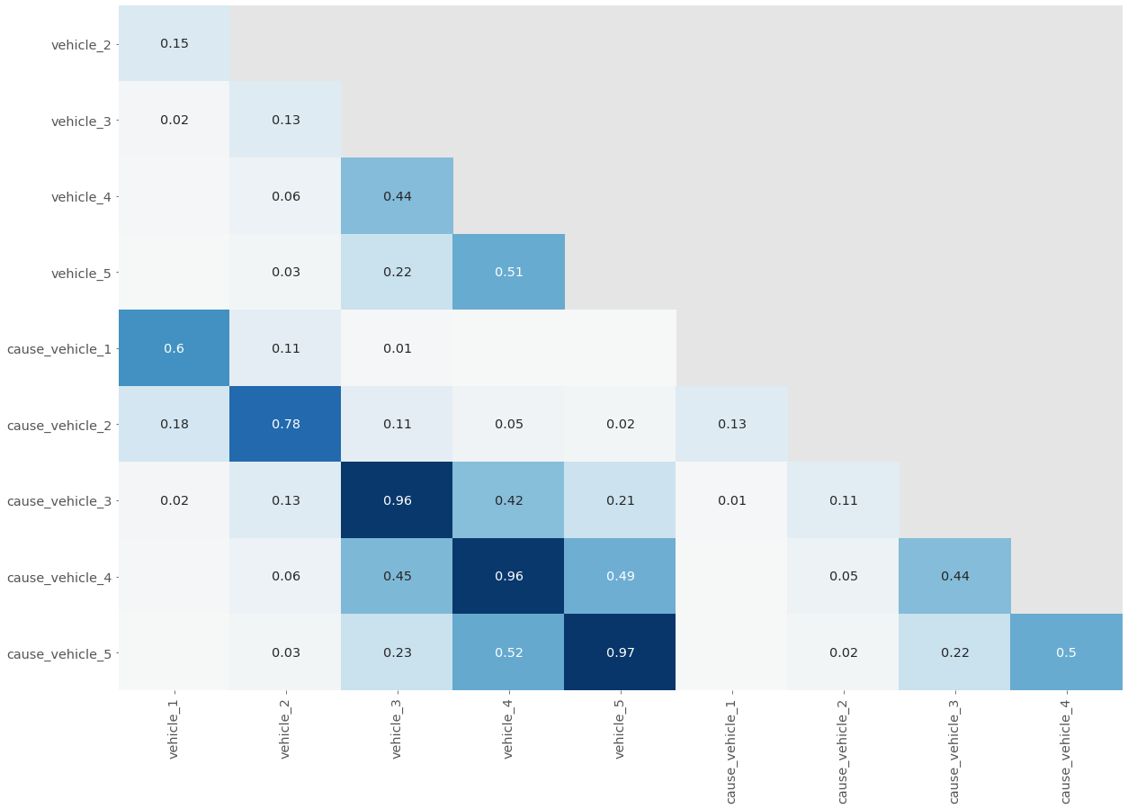
In our correlation plot:
- The “line of 1s” and the repeated values are removed so that it’s not visually overwhelming.
- Values very close to 0, where there is little to no relationship, aren’t labeled.
- Values close to 1 are dark blue and values close to -1 are light blue — the depth of color represents the strength of the relationship.
Analyzing Correlation in Missing Values
When a vehicle is in an accident, there is likely to be a cause, and vice-versa.
Let’s explore the variations in missing values from these five pairs of columns. We’ll create a dataframe that counts, for each pair:
- The number of values where the vehicle is missing when the cause is not missing.
- The number of values where the cause is missing when the vehicle is not missing.
col_labels = ['v_number', 'vehicle_missing', 'cause_missing']

vc_null_data = []

for v in range(1,6):
    v_col = 'vehicle_{}'.format(v)
    c_col = 'cause_vehicle_{}'.format(v)
    v_null = mvc[mvc[v_col].isnull() & mvc[c_col].notnull()].shape[0]
    c_null = mvc[mvc[v_col].notnull() & mvc[c_col].isnull()].shape[0]
    vc_null_data.append([v, v_null, c_null])

vc_null_df = pd.DataFrame(vc_null_data, columns=col_labels)
vc_null_df| v_number | vehicle_missing | cause_missing | |
|---|---|---|---|
| 0 | 1 | 204 | 24 |
| 1 | 2 | 3793 | 223 |
| 2 | 3 | 242 | 24 |
| 3 | 4 | 50 | 3 |
| 4 | 5 | 10 | 0 |
Finding The Most Common Value Across multiple Columns
The analysis we indicates that there are roughly 4,500 missing values across the 10 columns. The easiest option for handling these would be to drop the rows with missing values. This would mean losing almost 10% of the total data, which is something we ideally want to avoid.
A better option is to impute the data, like we did earlier. Because the data in these columns is text data, we can’t perform a numeric calculation to impute missing data.
One common option when imputing is to use the most common value to fill in data. Let’s look at the common values across these columns and see if we can use that to make a decision.
Let’s count the most common values for the cause set of columns. We’ll start by selecting only the columns containing the substring cause.
cause = mvc[[c for c in mvc.columns if "cause_" in c]]
cause.head()| cause_vehicle_1 | cause_vehicle_2 | cause_vehicle_3 | cause_vehicle_4 | cause_vehicle_5 | |
|---|---|---|---|---|---|
| 0 | Following Too Closely | Unspecified | NaN | NaN | NaN |
| 1 | Backing Unsafely | Unspecified | NaN | NaN | NaN |
| 2 | Following Too Closely | Unspecified | NaN | NaN | NaN |
| 3 | Glare | Passing Too Closely | NaN | NaN | NaN |
| 4 | Turning Improperly | Unspecified | NaN | NaN | NaN |
Next, we’ll stack the values into a single series object:
cause_1d = cause.stack()
cause_1d.head()
0 cause_vehicle_1 Following Too Closely
cause_vehicle_2 Unspecified
1 cause_vehicle_1 Backing Unsafely
cause_vehicle_2 Unspecified
2 cause_vehicle_1 Following Too Closely
dtype: objectYou may notice that the stacked version omits null values - this is fine, as we’re just interested in the most common non-null values.
Finally, we count the values in the series:
cause_counts = cause_1d.value_counts()
top10_causes = cause_counts.head(10)
top10_causes
Unspecified 57481
Driver Inattention/Distraction 17650
Following Too Closely 6567
Failure to Yield Right-of-Way 4566
Passing or Lane Usage Improper 3260
Passing Too Closely 3045
Backing Unsafely 3001
Other Vehicular 2523
Unsafe Lane Changing 2372
Turning Improperly 1590
dtype: int64The most common non-null value for the cause columns is Unspecified, which presumably indicates that the officer reporting the collision was unable to determine the cause for that vehicle.
Let’s identify the most common non-null value for the vehicle columns.
v_cols = [c for c in mvc.columns if c.startswith("vehicle")]
top10_vehicles = mvc[v_cols].stack().value_counts().head(10)
top10_vehicles
Sedan 33133
Station Wagon/Sport Utility Vehicle 26124
PASSENGER VEHICLE 16026
SPORT UTILITY / STATION WAGON 12356
Taxi 3482
Pick-up Truck 2373
TAXI 1892
Box Truck 1659
Bike 1190
Bus 1162
dtype: int64Filling Unknow values with a placeholder
The top “cause” is an "Unspecified" placeholder. This is useful instead of a null value as it makes the distinction between a value that is missing because there were only a certain number of vehicles in the collision versus one that is because the contributing cause for a particular vehicle is unknown.
The vehicles columns don’t have an equivalent, but we can still use the same technique. Here’s the logic we’ll need to do for each pair of vehicle/cause columns:
- For values where the vehicle is null and the cause is non-null, set the vehicle to
Unspecified. - For values where the cause is null and the vehicle is not-null, set the cause to
Unspecified.
def summarize_missing():
    v_missing_data = []

    for v in range(1,6):
        v_col = 'vehicle_{}'.format(v)
        c_col = 'cause_vehicle_{}'.format(v)

        v_missing = (mvc[v_col].isnull() & mvc[c_col].notnull()).sum()
        c_missing = (mvc[c_col].isnull() & mvc[v_col].notnull()).sum()

        v_missing_data.append([v, v_missing, c_missing])

    col_labels = columns=["vehicle_number", "vehicle_missing", "cause_missing"]
    return pd.DataFrame(v_missing_data, columns=col_labels)

summarize_missing()| vehicle_number | vehicle_missing | cause_missing | |
|---|---|---|---|
| 0 | 1 | 204 | 24 |
| 1 | 2 | 3793 | 223 |
| 2 | 3 | 242 | 24 |
| 3 | 4 | 50 | 3 |
| 4 | 5 | 10 | 0 |
for v in range(1,6):
    v_col = 'vehicle_{}'.format(v)
    c_col = 'cause_vehicle_{}'.format(v)
    mvc[v_col] = mvc[v_col].mask( mvc[v_col].isnull() & mvc[c_col].notnull(), 'Unspecified')
    mvc[c_col] = mvc[c_col].mask(mvc[v_col].notnull() & mvc[c_col].isnull(), "Unspecified")

summarize_missing()| vehicle_number | vehicle_missing | cause_missing | |
|---|---|---|---|
| 0 | 1 | 0 | 0 |
| 1 | 2 | 0 | 0 |
| 2 | 3 | 0 | 0 |
| 3 | 4 | 0 | 0 |
| 4 | 5 | 0 | 0 |
Missing data in the “location” column
Let’s view the work we’ve done across the past few screens by looking at the null correlation plot for the last 10 columns:
veh_cols = [c for c in mvc.columns if 'vehicle' in c]
plot_null_correlations(mvc[veh_cols])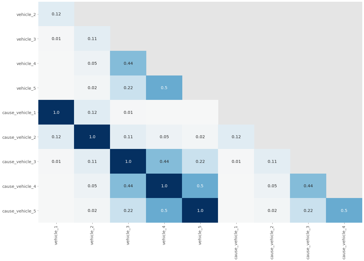
You can see the perfect correlation between each pair of vehicle/cause columns represented by 1.0 in each square, which means that there is a perfect relationship between the five pairs of vehicle/cause columns
Let’s now turn our focus to the final set of columns that contain missing values — the columns that relate to the location of the accident. We’ll start by looking at the first few rows to refamiliarize ourselves with the data:
loc_cols = ['borough', 'location', 'on_street', 'off_street', 'cross_street']
location_data = mvc[loc_cols]
location_data.head()| borough | location | on_street | off_street | cross_street | |
|---|---|---|---|---|---|
| 0 | MANHATTAN | (40.742832, -74.00771) | WEST 15 STREET | NaN | 10 AVENUE |
| 1 | BROOKLYN | (40.623714, -73.99314) | 16 AVENUE | NaN | 62 STREET |
| 2 | NaN | (40.591755, -73.9083) | BELT PARKWAY | NaN | NaN |
| 3 | QUEENS | (40.73602, -73.87954) | GRAND AVENUE | NaN | VANLOON STREET |
| 4 | BRONX | (40.884727, -73.89945) | NaN | 208 WEST 238 STREET | NaN |
Next, let’s look at counts of the null values in each column:
location_data.isnull().sum()borough 20646
location 3885
on_street 13961
off_street 44093
cross_street 29249
dtype: int64These columns have a lot of missing values! Keep in mind that all of these five columns represent the same thing — the location of the collision. We can potentially use the non-null values to impute some of the null values.
To see where we might be able to do this, let’s look for correlations between the missing values:
plot_null_correlations(location_data)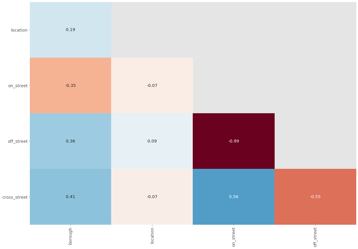
None of these columns have strong correlations except for off_street and on_street which have a near perfect negative correlation. That means for almost every row that has a null value in one column, the other has a non-null value and vice-versa.
The final way we’ll look at the null values in these columns is to plot a null matrix, but we’ll sort the data first. This will gather some of the null and non-null values together and make patterns more obvious:
sorted_location_data = location_data.sort_values(loc_cols)
plot_null_matrix(sorted_location_data)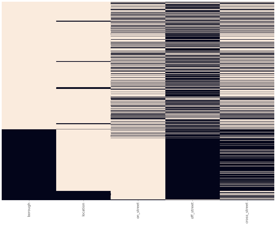
Let’s make some observations about the missing values across these columns:
- About two-thirds of rows have non-null values for
borough, but of those values that are missing, most have non-null values forlocationand one or more of thestreetname columns. - Less than one-tenth of rows have missing values in the
locationcolumn, but most of these have non-null values in one or more of thestreetname columns. - Most rows have a non-null value for either
on_streetoroff_street, and some also have a value forcross_street.
Combined, this means that we will be able to impute a lot of the missing values by using the other columns in each row. To do this, we can use geolocation APIs that take either an address or location coordinates, and return information about that location.
Imputing Location Data
sup_data = pd.read_csv('../datasets/supplemental_data.csv')
sup_data.head()| unique_key | location | on_street | off_street | borough | |
|---|---|---|---|---|---|
| 0 | 3869058 | NaN | NaN | NaN | NaN |
| 1 | 3847947 | NaN | NaN | NaN | NaN |
| 2 | 3914294 | NaN | BELT PARKWAY | NaN | BROOKLYN |
| 3 | 3915069 | NaN | NaN | NaN | NaN |
| 4 | 3923123 | NaN | NaN | NaN | NaN |
The supplemental data has five columns from our original data set — the unique_key that identifies each collision, and four of the five location columns. The cross_street column is not included because the geocoding APIs we used don’t include data on the nearest cross street to any single location.
Let’s take a look at a null matrix for the supplemental data:
plot_null_matrix(sup_data)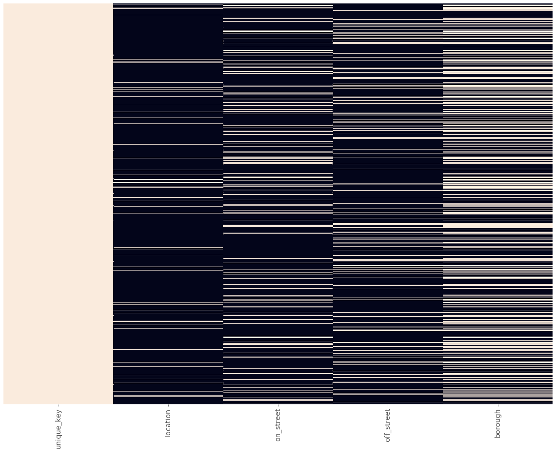
Apart from the unique_key column, you’ll notice that there are a lot more missing values than our main data set. This makes sense, as we didn’t prepare supplemental data where the original data set had non-null values.
mvc.unique_key.equals(sup_data.unique_key)Trueboth the original and supplemental data has the same values in the same order, we’ll be able to use Series.mask() to add our supplemental data to our original data.
location_cols = ['location', 'on_street', 'off_street', 'borough']
mvc[location_cols].isnull().sum()
location 3885
on_street 13961
off_street 44093
borough 20646
dtype: int64for c in location_cols:
mvc[c] = mvc[c].mask(mvc[c].isnull(), sup_data[c])
mvc[location_cols].isnull().sum()location 77
on_street 13734
off_street 36131
borough 232
dtype: int64we’ve imputed thousands of values to reduce the number of missing values across our data set. Let’s look at a summary of the null values
mvc.isnull().sum()unique_key 0
date 0
time 0
borough 232
location 77
on_street 13734
cross_street 29249
off_street 36131
pedestrians_injured 0
cyclist_injured 0
motorist_injured 0
total_injured 21
pedestrians_killed 0
cyclist_killed 0
motorist_killed 0
total_killed 1
vehicle_1 151
vehicle_2 8469
vehicle_3 54110
vehicle_4 57108
vehicle_5 57671
cause_vehicle_1 151
cause_vehicle_2 8469
cause_vehicle_3 54110
cause_vehicle_4 57108
cause_vehicle_5 57671
dtype: int64If we’d like to continue working with this data, we can:
- Drop the rows that had suspect values for
injuredandkilledtotals. - Clean the values in the
vehicle_1throughvehicle_5columns by analyzing the different values and merging duplicates and near-duplicates. - Analyze whether collisions are more likely in certain locations, at certain times, or for certain vehicle types.